Major topics covered in this chapter

Measures of location and spread; mean, standard deviation, variance
Normal and log-normal distributions; samples and populations
Sampling distribution of the mean; central limit theorem
Confidence limits and intervals
Presentation and rounding of results
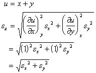
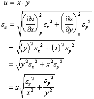
Propagation of errors in multi-stage experiments

Repeated measurements in analytical experiments in order to reveal the presence of random errors.

Table 2.1 Results of 50 determinations of nitrate ion concentration, in μg ml-1

Titration Data¶

The distribution of the results can most easily be appreciated by drawing a histogram

Summary of Titration Data¶

Posterior Plot of Mean¶

Posterior Plot of Sigma¶

Plot Comparison¶

Summary of Summary¶

The distribution of repeated measurements¶

standard deviation gives a measure of the spread of a set of results about the mean value, it does not indicate the shape of the distribution

The results can be summarised in a frequency table. The distribution of the results appreciated by drawing a histogram. This shows that the distribution of the measurements is roughly symmetrical about the mean, with the measurements clustered towards the centre.

$$ mean +- std $$

Although it cannot be proved that replicate values of a single analytical quantity are always normally distributed, there is considerable evidence that this assumption is generally at least approximately true. Moreover we shall see when we come to look at sample means that any departure of a population from normality is not usually important in the context of the statistical tests most frequently used.

Normal Distribution¶

Normal Distribution Mean = 0, 1, 2¶

PDF and CDF¶

Probability Estimation¶

Example 2.2.1¶

Log-normal distribution¶

In situations where one measurement is made on each of a number of specimens, distributions other than the normal distribution can also occur.
In particular the so-called log-normal distribution is frequently encountered.
For this distribution, frequency plotted against the logarithm of the concentration (or other characteristics) gives a normal distribution curve.
An example of a variable which has a log-normal distribution is the antibody concentration in human blood sera.

Definition of a ‘sample’¶

Sample in its statistical sense of a group of objects selected from the population of all such objects, for example a sample of 50 measurements of nitrate ion concentration from the (infinite) population of all such possible measurements, or a sample of healthy human adults chosen from the whole population in order to measure the concentration of serum albumin for each one.

The Commission on Analytical Nomenclature of the Analytical Chemistry Division of the International Union of Pure and Applied Chemistry has pointed out that confusion and ambiguity can arise if the term ‘sample’ is also used in its colloquial sense of the actual material being studied.
It recommends that the term ‘sample’ is confined to its statistical concept. Other words should be used to describe the material on which measurements are being made, in each case preceded by ‘test’, for example test solution or test extract.
We can then talk unambiguously of a sample of measurements on a test extract, or a sample of tablets from a batch.
A test portion from a population which varies with time, such as a river or circulating blood, should be described as a specimen.
Unfortunately this practice is by no means usual, so the term ‘sample’ remains in use for two related but distinct purposes.

Confidence limits of the mean for large samples¶

For 95% confidence limits, z 1.96 For 99% confidence limits, z 2.58 For 99.7% confidence limits, z 2.97

$$Standardised Normal Variable, z = {(x - mean)}$$

Confidence limits of the mean for large samples¶

Example 2.6.1 Calculate the 95% and 99% confidence limits of the mean for the nitrate ion concentration measurements in Table 2.1. From previous examples we have found that $\mu$ = 0.500 ,$\sigma$ = 0.0165 and n = 50. Using Eq. (2.6.3) gives the 95% confidence limits as: $$x +- 1.96 * s/ = 0.500 + 1.96 * 0.0165>250 = 0.500 ; 0.005 mg ml-1$$ and the 99% confidence limits as: x ; 2.58s>2n = 0.500 ; 2.58 * 0.01651>250 = 0.500 ; 0.006 mg ml-1

Confidence limits of the mean for large samples¶

Confidence limits of the mean for small samples¶

Significance tests

In a new method for determining selenourea in water the following values were obtained for tap water samples spiked with 50 ng ml1 of selenourea: 50.4, 50.7, 49.1, 49.0, 51.1 ng ml1

Propagation of random errors

The quantum yield of fluorescence, , of a material in solution is calculated from the expression: where the quantities involved are defined below, with an estimate of their relative standard deviations in brackets:

$$ f = {I_f}$$

$I_0$ incident light intensity (0.5%)
$I_f$ fluorescence intensity (2%)
e molar absorptivity (1%)
c concentration (0.2%)
l optical pathlength (0.2%)
k is an instrument constant. From Eq. (2.11.4), the relative standard deviation (RSD) of is given by:

	mean	sd	hpd_3%	hpd_97%	mcse_mean	mcse_sd	ess_mean	ess_sd	ess_bulk	ess_tail	r_hat
mean	0.500	0.002	0.495	0.504	0.0	0.0	1194.0	1192.0	1201.0	1072.0	1.0
sigma	0.017	0.002	0.014	0.020	0.0	0.0	1589.0	1565.0	1593.0	1124.0	1.0

	mean	sd	hpd_3%	hpd_97%	mcse_mean	mcse_sd	ess_mean	ess_sd	ess_bulk	ess_tail	r_hat
mean	100.471	0.374	99.799	101.202	0.012	0.008	997.0	997.0	1002.0	975.0	1.0
sigma	0.981	0.018	0.948	1.000	0.001	0.000	1270.0	1268.0	941.0	588.0	1.0

	mean	sd	hpd_3%	hpd_97%	mcse_mean	mcse_sd	ess_mean	ess_sd	ess_bulk	ess_tail	r_hat
mean	50.042	0.346	49.315	50.648	0.014	0.010	610.0	610.0	613.0	674.0	1.01
std	0.806	0.123	0.589	1.000	0.004	0.003	1063.0	956.0	796.0	489.0	1.01